TTT for Corrupted MNIST

Explore how test-time training can enhance model performance on corrupted MNIST data.

In this tutorial, we will explore how the original image rotation-based Test-Time Training (TTT) approach can improve model performance during inference when the data is corrupted by Gaussian noise, using the torch-ttt Engine functionality.

This notebook is designed to demonstrate how seamlessly test-time training approaches can be integrated through torch-ttt into existing training and testing pipelines, while also showcasing the significant performance improvements achievable when applying TTT on corrupted or out-of-distribution data.

Regular Model (without TTT)

Below, we will start by training regular networks on MNIST data and demonstrate how susceptible it is to noise introduced during testing, resulting in significantly lower accuracy when the noise is present.

Data and Model

Let’s start with some global parameters that we will use later.

import torch
import torchvision
import numpy as np
import random
import tqdm
import matplotlib.pyplot as plt

import torch.nn as nn
import torch.nn.functional as F
import torch.optim as optim

n_epochs = 1  # number of training epochs
batch_size_train = 64  # batch size during training
batch_size_test = 32  # batch size during training
learning_rate = 0.01  # training learning rate

random_seed = 7
torch.backends.cudnn.enabled = False
torch.manual_seed(random_seed)
random.seed(random_seed)
np.random.seed(random_seed)

# sphinx_gallery_thumbnail_path = '_static/images/examples/mnist_noisy.png'

We will employ a fairly shallow and simple model, consisting only of several convolutional and linear layers with LeakyReLU activations.

class Net(nn.Module):
    def __init__(self):
        super(Net, self).__init__()
        self.conv1 = nn.Conv2d(1, 10, kernel_size=5)
        self.conv2 = nn.Conv2d(10, 20, kernel_size=5)
        self.fc1 = nn.Linear(320, 50)
        self.fc2 = nn.Linear(50, 50)
        self.fc3 = nn.Linear(50, 10)
        self.activation = nn.LeakyReLU()

    def forward(self, x):
        x = self.activation(F.max_pool2d(self.conv1(x), 2))
        x = self.activation(F.max_pool2d(self.conv2(x), 2))
        x = x.view(-1, 320)
        x = self.activation(self.fc1(x))
        x = self.activation(self.fc2(x))
        x = self.fc3(x)
        return F.log_softmax(x, dim=-1)

For training and testing data, we will use the standard train/test MNIST split, which consists of roughly 60,000 samples for training and 10,000 for testing, and we will normalize the data.

train_loader = torch.utils.data.DataLoader(
    torchvision.datasets.MNIST(
        "./MNIST/",
        train=True,
        download=True,
        transform=torchvision.transforms.Compose(
            [
                torchvision.transforms.ToTensor(),
                torchvision.transforms.Normalize((0.1307,), (0.3081,)),
            ]
        ),
    ),
    batch_size=batch_size_train,
    shuffle=False,
)

test_loader = torch.utils.data.DataLoader(
    torchvision.datasets.MNIST(
        "./MNIST/",
        train=False,
        download=True,
        transform=torchvision.transforms.Compose(
            [
                torchvision.transforms.ToTensor(),
                torchvision.transforms.Normalize((0.1307,), (0.3081,)),
            ]
        ),
    ),
    batch_size=batch_size_test,
    shuffle=False,
)

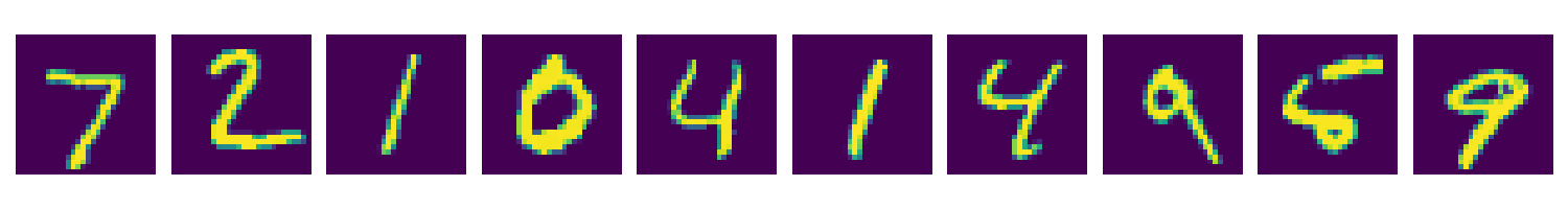
First, let’s visualize 10 random images from the clean MNIST test set. As we can see, the digits are clearly visible and distinctive.

images, _ = next(iter(test_loader))
fig, axes = plt.subplots(1, 10, figsize=(15, 2))
for ax, img in zip(axes, images[:10, 0]):
    ax.imshow(img, cmap="viridis")
    ax.axis("off")
plt.tight_layout()
plt.show()

Training and Testing

Following a rather simple training pipeline, we train our model for one epoch and then evaluate it on the test set.

network = Net()
optimizer = optim.Adam(network.parameters(), lr=learning_rate)


def train():
    network.train()
    correct = 0
    with tqdm.tqdm(total=len(train_loader), desc="Train") as pbar:
        for batch_idx, (data, target) in enumerate(train_loader):
            optimizer.zero_grad()
            output = network(data)
            pred = output.data.max(1, keepdim=True)[1]
            correct += pred.eq(target.data.view_as(pred)).sum().item()
            loss = F.nll_loss(output, target)
            loss.backward()
            optimizer.step()

            if (batch_idx + 1) % 150 == 0:
                pbar.update(150)

        pbar.set_postfix(acc=correct / len(train_loader.dataset))


def test():
    network.eval()
    correct = 0
    with torch.no_grad():
        with tqdm.tqdm(total=len(test_loader), desc="Test") as pbar:
            for batch_idx, (data, target) in enumerate(test_loader):
                output = network(data)
                pred = output.data.max(1, keepdim=True)[1]
                correct += pred.eq(target.data.view_as(pred)).sum().item()
                if (batch_idx + 1) % 100 == 0:
                    pbar.update(100)

            accuracy = 100.0 * correct / len(test_loader.dataset)
            pbar.set_postfix(acc=accuracy)

As we can see below, our model achieves roughly 95% accuracy on both the train and test sets.

for _ in range(n_epochs):
    train()
test()

Train:   0%|          | 0/938 [00:00<?, ?it/s]
Train:  16%|█▌        | 150/938 [00:01<00:10, 78.77it/s]
Train:  32%|███▏      | 300/938 [00:03<00:07, 80.58it/s]
Train:  48%|████▊     | 450/938 [00:05<00:06, 80.93it/s]
Train:  64%|██████▍   | 600/938 [00:07<00:04, 79.36it/s]
Train:  80%|███████▉  | 750/938 [00:09<00:02, 80.11it/s]
Train:  96%|█████████▌| 900/938 [00:11<00:00, 81.39it/s]
Train:  96%|█████████▌| 900/938 [00:11<00:00, 81.39it/s, acc=0.947]
Train:  96%|█████████▌| 900/938 [00:11<00:00, 77.59it/s, acc=0.947]

Test:   0%|          | 0/313 [00:00<?, ?it/s]
Test:  32%|███▏      | 100/313 [00:00<00:01, 194.99it/s]
Test:  64%|██████▍   | 200/313 [00:01<00:00, 186.67it/s]
Test:  96%|█████████▌| 300/313 [00:01<00:00, 184.14it/s]
Test:  96%|█████████▌| 300/313 [00:01<00:00, 184.14it/s, acc=97.2]
Test:  96%|█████████▌| 300/313 [00:01<00:00, 177.92it/s, acc=97.2]

Evaluating on noisy test

Now, let’s add a significant amount of Gaussian noise to our input images, which will make the classification task significantly more challenging. Let’s plot how they look.

images, _ = next(iter(test_loader))
fig, axes = plt.subplots(1, 10, figsize=(15, 2))
for ax, img in zip(axes, images[:10, 0]):
    noisy_img = img + 2 * torch.randn(img.shape)
    ax.imshow(noisy_img, cmap="viridis")
    ax.axis("off")
plt.tight_layout()
plt.show()

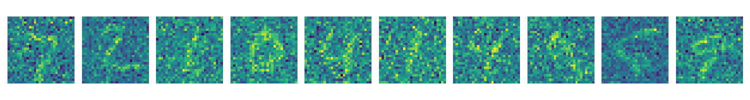
Since the model was not exposed to this type of corruption during training, these new corrupted inputs can be considered out-of-distribution. As a result, the model shows significantly lower accuracy on these inputs. As we can see below, the accuracy drops from roughly 95% to below 60%.

network.eval()
correct = 0
with torch.no_grad():
    with tqdm.tqdm(total=len(test_loader), desc="Test") as pbar:
        for batch_idx, (data, target) in enumerate(test_loader):
            data += 2 * torch.randn(data.shape)
            output = network(data)
            pred = output.data.max(1, keepdim=True)[1]
            correct += pred.eq(target.data.view_as(pred)).sum().item()
            if (batch_idx + 1) % 100 == 0:
                pbar.update(100)

        accuracy = 100.0 * correct / len(test_loader.dataset)
        pbar.set_postfix(acc=accuracy)

Test:   0%|          | 0/313 [00:00<?, ?it/s]
Test:  32%|███▏      | 100/313 [00:00<00:01, 168.92it/s]
Test:  64%|██████▍   | 200/313 [00:01<00:00, 168.65it/s]
Test:  96%|█████████▌| 300/313 [00:01<00:00, 167.86it/s]
Test:  96%|█████████▌| 300/313 [00:01<00:00, 167.86it/s, acc=40.2]
Test:  96%|█████████▌| 300/313 [00:01<00:00, 161.32it/s, acc=40.2]

Optimized Model (with TTT)

Now, let’s employ the original TTT approach to improve the performance on these noisy inputs. We will use the TTTEngine class, which encapsulates the mechanism of TTT’s image rotation-based self-supervised loss and gradient optimization during inference.

from torch_ttt.engine.ttt_engine import TTTEngine  # noqa: E402

Test-Time Training (TTT) leverages a self-supervised auxiliary task to adapt the model to unseen data distributions during inference. In the training phase, the model is optimized jointly for the primary task and the auxiliary self-supervised task—here, image rotation prediction. This involves learning shared features through the encoder \(\theta_{e}\) while the supervised task head \(\theta_{m}\) (e.g. classification) and self-supervised task head \(\theta_{s}\) (rotation angle prediction) specialize in their respective objectives.

During testing, the model adapts to out-of-distribution or noisy inputs by optimizing the self-supervised loss associated with the auxiliary task, enhancing the robustness of primary task predictions. Our TTTEngine class seamlessly implements both the training and testing behaviors of the TTT framework, as demonstrated in the example below. For a more detailed overview of the TTT framework, please refer to the original webpage and slides.

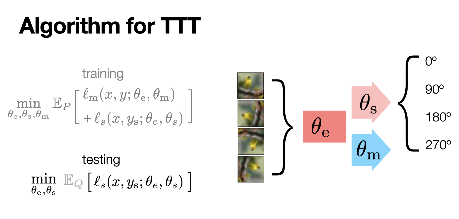
Figure 1. Overview of the TTT framework. It incorporates joint training with supervised and self-supervised tasks (image rotation prediction) and adapts during inference by optimizing the self-supervised loss for improved predictions.

Training and Testing

We need to add only a couple of new lines to our original training and testing functions to introduce TTT into the existing pipelines. Below, we add a comment for each line that was either newly added or modified.

network = Net()
engine = TTTEngine(network, "fc2")  # create an engine object
optimizer = optim.Adam(engine.parameters(), lr=learning_rate)  # optimize the engine, not model


def train():
    engine.train()  # switch engine to .train() mode
    correct = 0
    with tqdm.tqdm(total=len(train_loader), desc="Train") as pbar:
        for batch_idx, (data, target) in enumerate(train_loader):
            optimizer.zero_grad()
            output, loss_ttt = engine(data)  # run inferece with engine
            pred = output.data.max(1, keepdim=True)[1]
            correct += pred.eq(target.data.view_as(pred)).sum().item()
            loss = (
                F.nll_loss(output, target) + 0.35 * loss_ttt
            )  # add self-supervised loss to the total loss
            loss.backward()
            optimizer.step()

            if (batch_idx + 1) % 150 == 0:
                pbar.update(150)

        pbar.set_postfix(acc=correct / len(train_loader.dataset))

As shown below, the accuracy of the underlying model remains the same for both the original training and the TTT-based training.

for _ in range(n_epochs):
    train()
test()  # evaluation of the underlying model, without TTT

Train:   0%|          | 0/938 [00:00<?, ?it/s]
Train:  16%|█▌        | 150/938 [00:02<00:15, 50.34it/s]
Train:  32%|███▏      | 300/938 [00:05<00:12, 50.53it/s]
Train:  48%|████▊     | 450/938 [00:08<00:09, 51.81it/s]
Train:  64%|██████▍   | 600/938 [00:11<00:06, 51.57it/s]
Train:  80%|███████▉  | 750/938 [00:14<00:03, 51.72it/s]
Train:  96%|█████████▌| 900/938 [00:17<00:00, 52.29it/s]
Train:  96%|█████████▌| 900/938 [00:18<00:00, 52.29it/s, acc=0.946]
Train:  96%|█████████▌| 900/938 [00:18<00:00, 49.71it/s, acc=0.946]

Test:   0%|          | 0/313 [00:00<?, ?it/s]
Test:  32%|███▏      | 100/313 [00:00<00:01, 186.32it/s]
Test:  64%|██████▍   | 200/313 [00:01<00:00, 196.60it/s]
Test:  96%|█████████▌| 300/313 [00:01<00:00, 201.23it/s]
Test:  96%|█████████▌| 300/313 [00:01<00:00, 201.23it/s, acc=96.3]
Test:  96%|█████████▌| 300/313 [00:01<00:00, 191.07it/s, acc=96.3]

Evaluating on noisy test

Now, let’s return to the evaluation of the model on inputs when a significant amount of noise is introduced. As we saw before, the original model demonstrated a significant drop in accuracy when the noise was introduced. Below, we will enable test-time training optimization during inference (which happens in the engine’s .forward() function) to improve the model’s performance on noisy images. As with the training, we will mark the changed/modified lines with a comment.

def ttt_test():
    engine.eval()  # switch engine to .eval() mode
    correct = 0
    with tqdm.tqdm(total=len(test_loader), desc="Test") as pbar:
        for batch_idx, (data, target) in enumerate(test_loader):
            data += 2 * torch.randn(data.shape)
            output, _ = engine(data)  # run inferece with engine
            pred = output.data.max(1, keepdim=True)[1]
            correct += pred.eq(target.data.view_as(pred)).sum().item()
            if (batch_idx + 1) % 100 == 0:
                pbar.update(100)

        accuracy = 100.0 * correct / len(test_loader.dataset)
        pbar.set_postfix(acc=accuracy)

The engine’s optimization_parameters dictionary stores the parameters used for optimization. Below, we modify the number of optimization steps to demonstrate how accuracy improves as the number of steps increases. As shown, the TTT engine with 3 optimization iterations improves the accuracy from ~54% for the original model by almost 15%, and further improvements can be achieved with more optimization steps.

print("### No optimization ###")
engine.optimization_parameters["num_steps"] = 0
ttt_test()

### No optimization ###

Test:   0%|          | 0/313 [00:00<?, ?it/s]
Test:  32%|███▏      | 100/313 [00:00<00:01, 156.44it/s]
Test:  64%|██████▍   | 200/313 [00:01<00:00, 158.70it/s]
Test:  96%|█████████▌| 300/313 [00:01<00:00, 148.52it/s]
Test:  96%|█████████▌| 300/313 [00:02<00:00, 148.52it/s, acc=60.4]
Test:  96%|█████████▌| 300/313 [00:02<00:00, 144.36it/s, acc=60.4]

print("### Number of optimization steps: 1 ###")
engine.optimization_parameters["num_steps"] = 1
ttt_test()

### Number of optimization steps: 1 ###

Test:   0%|          | 0/313 [00:00<?, ?it/s]
Test:  32%|███▏      | 100/313 [00:01<00:03, 68.10it/s]
Test:  64%|██████▍   | 200/313 [00:03<00:01, 65.78it/s]
Test:  96%|█████████▌| 300/313 [00:04<00:00, 64.77it/s]
Test:  96%|█████████▌| 300/313 [00:04<00:00, 64.77it/s, acc=62.9]
Test:  96%|█████████▌| 300/313 [00:04<00:00, 62.75it/s, acc=62.9]

print("### Number of optimization steps: 2 ###")
engine.optimization_parameters["num_steps"] = 2
ttt_test()

### Number of optimization steps: 2 ###

Test:   0%|          | 0/313 [00:00<?, ?it/s]
Test:  32%|███▏      | 100/313 [00:02<00:04, 47.99it/s]
Test:  64%|██████▍   | 200/313 [00:04<00:02, 47.49it/s]
Test:  96%|█████████▌| 300/313 [00:06<00:00, 45.60it/s]
Test:  96%|█████████▌| 300/313 [00:06<00:00, 45.60it/s, acc=64.5]
Test:  96%|█████████▌| 300/313 [00:06<00:00, 44.25it/s, acc=64.5]

print("### Number of optimization steps: 3 ###")
engine.optimization_parameters["num_steps"] = 3
ttt_test()

### Number of optimization steps: 3 ###

Test:   0%|          | 0/313 [00:00<?, ?it/s]
Test:  32%|███▏      | 100/313 [00:03<00:06, 31.49it/s]
Test:  64%|██████▍   | 200/313 [00:05<00:03, 34.87it/s]
Test:  96%|█████████▌| 300/313 [00:08<00:00, 36.46it/s]
Test:  96%|█████████▌| 300/313 [00:08<00:00, 36.46it/s, acc=65.4]
Test:  96%|█████████▌| 300/313 [00:08<00:00, 34.28it/s, acc=65.4]