ImageNet Robustness with TENT

Discover how test-time training can improve model performance on corrupted versions of ImageNet using torch-ttt.

In this tutorial, we demonstrate how test-time adaptation methods such as Tent can help restore accuracy when evaluating models on ImageNet-C, a corrupted variant of the ImageNet dataset. We leverage the torch-ttt library for easy and flexible integration.

print("Uncomment the line below to install torch-ttt if you're running this in Colab")
# !pip install git+https://github.com/nikitadurasov/torch-ttt.git

Uncomment the line below to install torch-ttt if you're running this in Colab

Helper Functions

Data Preparation

We will work with the ImageNet dataset, using both the clean validation set and the corrupted validation set from ImageNet-C. The corrupted version includes various types of distortions, such as noise, blur, and weather effects. For this tutorial, we’ll focus on a single corruption type: pixelation.

Let’s start by downloading both the clean and corrupted versions of the ImageNet validation set.

import os

# Download and extract clean ImageNet validation set
os.system("gdown 1Q6wQbNZMF0XdopzQGePDQAqVusMpbKxI && tar -xzf imagenet_clean.tar.gz")

# Download and extract corrupted ImageNet validation set
os.system("gdown 1AeMUO_6M0F0E7AOBxpb97svMXAwjtyXf && tar -xzf imagenet_corrupted.tar.gz")

0

… and importing the necessary libraries.

import torch
import torchvision.datasets as datasets
import torchvision.transforms as transforms
import torch.nn as nn
import torch.nn.functional as F
import time
import json
import urllib.request
import matplotlib.pyplot as plt
from torchvision import models
from torchvision.models import resnet50, ResNet50_Weights

os.environ['TORCH_HOME'] = './weights'
os.makedirs(os.environ['TORCH_HOME'], exist_ok=True)

# sphinx_gallery_thumbnail_path = '_static/images/examples/imagenet_corrupted.png'

Utility Classes

Later in the tutorial, we will use the following helper classes and functions to track and visualize the progress of our model evaluation on both the clean and corrupted versions of ImageNet, allowing us to observe the differences in performance.

class AverageMeter(object):
    def __init__(self, name, fmt=':f'):
        self.name = name
        self.fmt = fmt
        self.reset()

    def reset(self):
        self.val = 0
        self.avg = 0
        self.sum = 0
        self.count = 0

    def update(self, val, n=1):
        self.val = val
        self.sum += val * n
        self.count += n
        self.avg = self.sum / self.count

    def __str__(self):
        fmtstr = '{name} {val' + self.fmt + '} ({avg' + self.fmt + '})'
        return fmtstr.format(**self.__dict__)

class ProgressMeter(object):
    def __init__(self, num_batches, meters, prefix=""):
        self.batch_fmtstr = self._get_batch_fmtstr(num_batches)
        self.meters = meters
        self.prefix = prefix

    def display(self, batch):
        entries = [self.prefix + self.batch_fmtstr.format(batch)]
        entries += [str(meter) for meter in self.meters]
        print('\t'.join(entries))

    def display_summary(self):
        entries = [" *"]
        entries += [str(meter) for meter in self.meters]
        print(' '.join(entries))

    def _get_batch_fmtstr(self, num_batches):
        num_digits = len(str(num_batches // 1))
        fmt = '{:' + str(num_digits) + 'd}'
        return '[' + fmt + '/' + fmt.format(num_batches) + ']'

# Human-readable labels
synset_to_name = json.load(urllib.request.urlopen(
    "https://raw.githubusercontent.com/anishathalye/imagenet-simple-labels/master/imagenet-simple-labels.json"
))
human_readable_labels = synset_to_name


def visualize_samples(dataset):
    """Visualize a few samples from the dataset and return the plot."""
    mean = torch.tensor([0.485, 0.456, 0.406]).view(3,1,1)
    std = torch.tensor([0.229, 0.224, 0.225]).view(3,1,1)

    images, labels = zip(*[dataset[i] for i in range(0, len(dataset), len(dataset) // 15)])
    images = [img * std + mean for img in images]

    fig, axes = plt.subplots(3, 5, figsize=(12, 7))
    for ax, img, label in zip(axes.flatten(), images, labels):
        ax.imshow(img.permute(1, 2, 0).clip(0, 1))
        ax.set_title(human_readable_labels[label], fontsize=8)
        ax.axis('off')
    plt.tight_layout()
    return fig

Accuracy and Validation Function

def accuracy(output, target, topk=(1,)):
    maxk = max(topk)
    batch_size = target.size(0)

    _, pred = output.topk(maxk, 1, True, True)
    pred = pred.t()
    correct = pred.eq(target.view(1, -1).expand_as(pred))

    res = []
    for k in topk:
        correct_k = correct[:k].reshape(-1).float().sum(0, keepdim=True)
        res.append(correct_k.mul_(100.0 / batch_size))
    return res

def validate(val_loader, model, criterion, device, ttt=False):
    batch_time = AverageMeter('Time', ':6.3f')
    losses = AverageMeter('Loss', ':.4e')
    top1 = AverageMeter('Acc@1', ':6.2f')
    top5 = AverageMeter('Acc@5', ':6.2f')
    progress = ProgressMeter(len(val_loader), [batch_time, losses, top1, top5], prefix='Test: ')

    model.eval()
    end = time.time()

    for i, (images, target) in enumerate(val_loader):
        images = images.to(device)
        target = target.to(device)

        output = model(images)[0] if ttt else model(images)
        loss = criterion(output, target)

        acc1, acc5 = accuracy(output, target, topk=(1, 5))
        losses.update(loss.item(), images.size(0))
        top1.update(acc1[0], images.size(0))
        top5.update(acc5[0], images.size(0))

        batch_time.update(time.time() - end)
        end = time.time()

        if i % 100 == 0:
            progress.display(i + 1)

    progress.display_summary()
    return float(top1.avg.item())

Clean Data Evaluation

Clean ImageNet Validation Set

First, let’s take a look at the clean validation set. We’ll visualize a few sample images. As you can see, the images are clear, and it’s relatively easy to recognize the objects they depict.

transform = transforms.Compose([
    transforms.Resize(256),
    transforms.CenterCrop(224),
    transforms.ToTensor(),
    transforms.Normalize(mean=[0.485, 0.456, 0.406], std=[0.229, 0.224, 0.225])
])

val_dataset = datasets.ImageFolder("./imagenet_clean", transform=transform)
val_loader = torch.utils.data.DataLoader(val_dataset, batch_size=32, shuffle=True, num_workers=8, pin_memory=True)

visualize_samples(val_dataset)

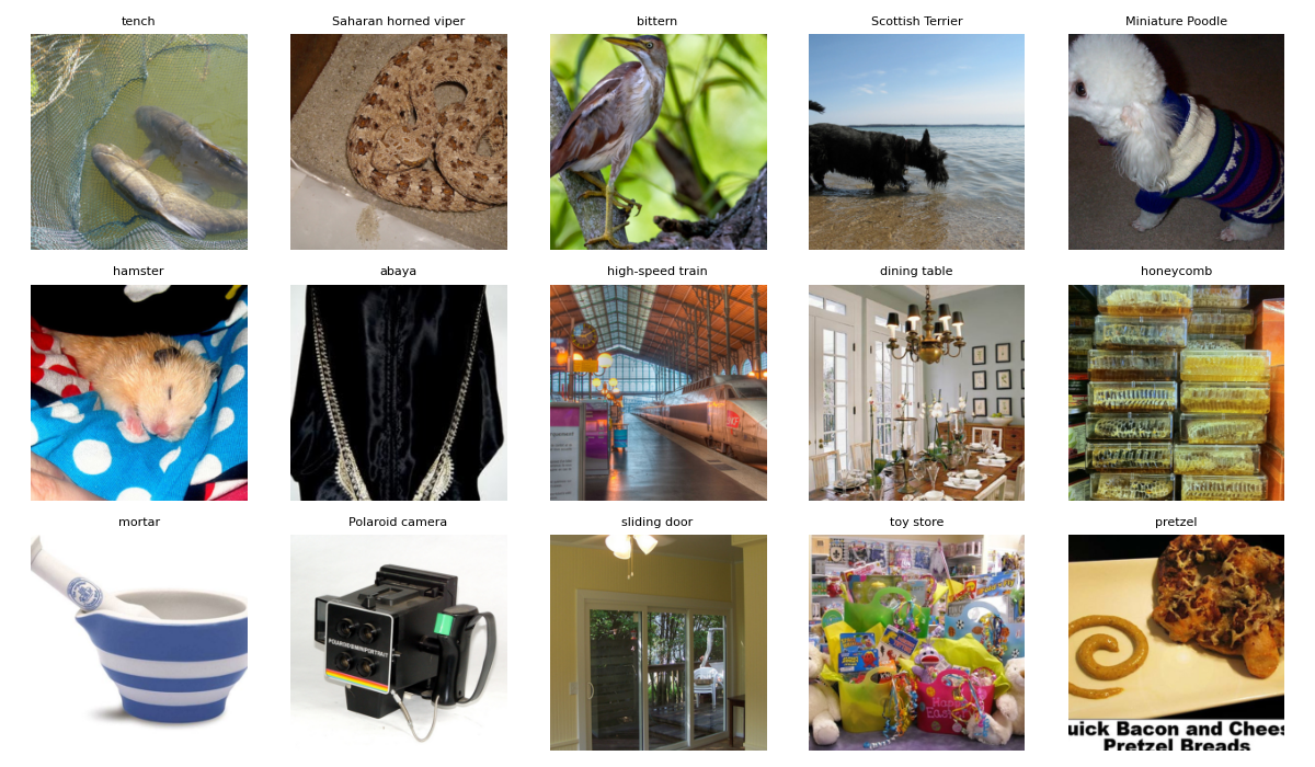
<Figure size 1200x700 with 15 Axes>

Pretrained Model Evaluation on Clean Data

Now, let’s load a pretrained ResNet-50 model and evaluate its performance on the clean validation set. We’ll use the torchvision library to load the model. The resulting accuracy, around 77%, aligns with the official accuracy reported by torchvision.

device = "cuda" if torch.cuda.is_available() else "cpu"
criterion = nn.CrossEntropyLoss().to(device)
model = resnet50(weights=ResNet50_Weights.IMAGENET1K_V1).to(device)
model.eval()

acc_clean = validate(val_loader, model, criterion, device)
print(f"Clean Accuracy: {acc_clean:.2f}%")

/scratch/cvlab/home/durasov/miniconda/envs/torch_ttt/lib/python3.10/site-packages/torch/hub.py:846: UserWarning: TORCH_MODEL_ZOO is deprecated, please use env TORCH_HOME instead
  warnings.warn(
Test: [  1/157] Time  1.066 ( 1.066)    Loss 1.0837e+00 (1.0837e+00)    Acc@1  71.88 ( 71.88)   Acc@5  96.88 ( 96.88)
Test: [101/157] Time  0.053 ( 0.063)    Loss 1.2988e+00 (9.5816e-01)    Acc@1  65.62 ( 76.61)   Acc@5  90.62 ( 93.35)
 * Time  0.013 ( 0.060) Loss 1.6625e-01 (9.2224e-01) Acc@1 100.00 ( 77.32) Acc@5 100.00 ( 93.36)
Clean Accuracy: 77.32%

Corrupted Data Evaluation

Corrupted ImageNet Validation Set

Now, let’s take a look at the corrupted validation set. We’ll visualize a few sample images as well. As you can see, the images are distorted, making it more difficult to recognize the objects they contain. In this example, we use pixelated images as the corruption type, which, as we’ll see, has a significant impact on the model’s performance.

corrupted_dataset = datasets.ImageFolder("./imagenet_corrupted", transform=transform)
corrupted_loader = torch.utils.data.DataLoader(corrupted_dataset, batch_size=32, shuffle=True, num_workers=8, pin_memory=True)

visualize_samples(corrupted_dataset)

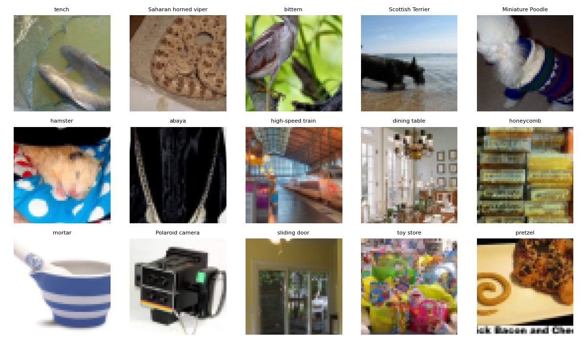
<Figure size 1200x700 with 15 Axes>

Pretrained Model Evaluation on Corrupted Data

Let’s evaluate the pretrained model on the corrupted validation set. As expected, the accuracy drops significantly—from 77% to around 20%—indicating that the model struggles to recognize objects in distorted images.

acc_corrupted = validate(corrupted_loader, model, criterion, device)
print(f"Corrupted Accuracy: {acc_corrupted:.2f}%")

Test: [  1/157] Time  0.469 ( 0.469)    Loss 3.4536e+00 (3.4536e+00)    Acc@1  28.12 ( 28.12)   Acc@5  53.12 ( 53.12)
Test: [101/157] Time  0.053 ( 0.058)    Loss 3.5986e+00 (4.3267e+00)    Acc@1  34.38 ( 23.08)   Acc@5  56.25 ( 43.44)
 * Time  0.013 ( 0.056) Loss 4.9279e+00 (4.3666e+00) Acc@1  25.00 ( 22.70) Acc@5  25.00 ( 43.08)
Corrupted Accuracy: 22.70%

Optimized Inference with torch-ttt

Test-Time Adaptation with Tent

As we’ve seen, image corruptions can significantly degrade model performance. To tackle this issue, we can use test-time adaptation techniques. In this example, we’ll demonstrate how to apply TENT (Test-time Entropy Minimization), which adapts the model to the input data during inference.

TENT works by minimizing the entropy of the model’s predictions, encouraging more confident outputs. During inference, the model produces a probability distribution over the classes. TENT computes the entropy of this distribution, then calculates gradients with respect to the parameters of the normalization layers (e.g., BatchNorm) and updates their affine parameters accordingly. This adaptation is performed for a set number of steps, allowing the model to better align with the current input distribution.

Using TENT with torch-ttt is straightforward: simply create a TentEngine instance and provide it with the model and optimization parameters such as the learning rate and number of adaptation steps. Even with just a single adaptation step, we observe a notable improvement in accuracy—about 10%—on corrupted ImageNet data compared to the original pretrained ResNet-50. Further tuning of the optimization parameters can lead to even better results.

from torch_ttt.engine.tent_engine import TentEngine

engine = TentEngine(
    model,
    optimization_parameters={
        "lr": 2e-3,
        "num_steps": 1
    }
)
engine.eval()

acc_tent = validate(corrupted_loader, engine, criterion, device, ttt=True)
print(f"Corrupted Accuracy with Tent: {acc_tent:.2f}%")

Test: [  1/157] Time  0.648 ( 0.648)    Loss 7.0112e+00 (7.0112e+00)    Acc@1  25.00 ( 25.00)   Acc@5  40.62 ( 40.62)
Test: [101/157] Time  0.194 ( 0.199)    Loss 3.1544e+00 (5.0462e+00)    Acc@1  46.88 ( 31.65)   Acc@5  78.12 ( 55.26)
 * Time  0.062 ( 0.196) Loss 8.7884e+00 (5.0529e+00) Acc@1  12.50 ( 31.24) Acc@5  12.50 ( 54.72)
Corrupted Accuracy with Tent: 31.24%